Interpreting Connectivity Scores and the Connectivity Matrix
You may also find user manual, guidance on applying the Connectivity Tool or understanding the data useful.
Key points
The Connectivity Tool gives each square a connectivity score from 0 to 100. The score helps users understand how well-connected a square is to locations of interest by walking and wheeling, cycling and public transport, compared with other squares across England and Wales.
The Connectivity Matrix is a set of tables that help users judge whether a square’s connectivity score is high or low for its destination type, transport mode, and how urban or rural the square is.
When interpreting the connectivity score, remember that:
- The score is a relative measure, not an absolute measure of connectivity – it shows how places compare to other places.
- A score of 50 does not mean a location has average connectivity.
- Scores should not be directly compared across different transport modes or destinations.
- The Connectivity Matrix can be used to help users compare a square with squares of the same rural-urban class.
- The score should be used alongside local evidence, site knowledge and professional judgement.
- Driving is not included in the overall connectivity score, although users can view scores for car-based journeys separately.
What does the connectivity score show?
Each square receives a score between 0 and 100. A higher score means the square is better-connected relative to other squares. A lower score means it is less well-connected relative to other squares.
Connectivity scores for each square are calculated as a percentage relative to the highest-scoring square in England and Wales, which is 100.
More detail on how the scores are calculated is available on the Understand the Data page.
What does the connectivity score not show?
The connectivity score does not give a final judgement on whether a location is suitable for development, investment or a transport intervention. It is one source of evidence.
The score does not currently measure:
- the quality of walking, wheeling, cycling or public transport routes, such as footway width, surface condition, lighting, segregated cycling facilities or step-free access;
- the cost or affordability of travel;
- service reliability or crowding;
- the specific travel needs of different people or groups; or
- electric bicycles or other assisted modes of transport.
For these reasons, the score should always be used alongside local evidence, professional judgement and other material considerations.
How should connectivity scores be interpreted?
Connectivity scores should always be interpreted comparatively. This is because the score tells users how a square’s connectivity compares to other squares, rather than whether its connectivity is “good” or “bad” in isolation.
For example, a square’s score may look low when compared to all scores nationally, but it could be relatively high for a rural area. Similarly, a score may look high nationally, but it may be low for a dense urban area.
This is why users should interpret the score in context. The most useful comparison is often with similar types of place, rather than with all places in England and Wales. This guidance proposes using rural-urban classifications (RUCs) as one of the ways to compare similar places. More detail is given later in this guidance page.
Does a score of 50 mean a location has average connectivity?
No. A score of 50 does not mean that a location has average connectivity.
The connectivity score is not a simple scale where 0 is the worst, 100 is the best, and 50 is the average.
The same connectivity score can mean different things depending on how other squares perform. For example, a score of 50 can be relatively well-connected, or poorly connected, depending on:
- the transport mode being considered;
- the destination being considered; and
- the rural-urban classification of the location.
Users should therefore avoid interpreting a connectivity score on its own. They should use the relevant tables in the Connectivity Matrix (detailed below) to understand where the square’s score sits in the wider distribution.
Can scores be compared across transport modes or destinations?
Scores for different transport modes or destinations should not be directly compared with each other. Each square’s score is calculated relative to other squares for a specific transport mode or destination – so comparison between destinations or modes does not provide meaningful information.
As an example, a square of interest may have:
- a score of 60 for access to education;
- a score of 70 for access to health services.
However, this does not automatically mean the square of interest is better connected to health services (70) than to education (60). This is because the other squares may score significantly higher than 70 for access to health services, meaning the square of interest’s score of 70 would be relatively worse. Each square needs to be interpreted against its own destination.
The same applies to transport modes. A location may have a walking score of 60 and a public transport score of 50. This does not automatically mean it is better connected by walking than by public transport. Each square should be interpreted against its own transport mode.
What is the Connectivity Matrix?
The Connectivity Matrix is a set of tables that help users judge whether a square’s connectivity score is high or low for its destination type, transport mode, and how urban or rural the place is.
This allows users to compare a location with similar places, rather than comparing it with all places nationally.
The Matrix shows percentile thresholds for different combinations of:
- rural-urban classification;
- transport mode;
- destination type;
The exact rural-urban classifications used in the Matrix are described in more detail later in this guidance.
What do the percentiles in the Connectivity Matrix mean?
The Connectivity Matrix uses percentiles. These indicate the percentage of Output Areas which have a lower or higher connectivity score.
For example:
- A square with a connectivity score at the 20th percentile threshold has a higher connectivity score than only 20% of Output Areas, meaning its score is lower than 80% of Output Areas;
- A square with a connectivity score at the 90th percentile threshold has a higher connectivity score than 90% of Output Areas, meaning its score is lower than only 10% of Output Areas.
This means:
- the 20th percentile is in the bottom 20%;
- the 50th percentile is the average;
- the 90th percentile is in the top 10%.
Users should focus on where a score sits in the relevant distribution, rather than on the connectivity score in isolation. For example, if the square of interest is in an “Urban major conurbation”, then the first column of Connectivity Matrix tables is the most relevant.
Which comparison should I use?
Different tables in the Connectivity Matrix answer different questions. Users should choose the right table for the question they are asking.
| Question | Best Table |
|---|---|
| How does my square compare to squares of the same rural-urban classification? | Connectivity Matrix |
| How does my square compare to other squares of the same destination type, nationally? | Table A |
| How does my square compare to other squares of the same transport mode, nationally? | Table B |
The Connectivity Matrix is most useful when users want to understand whether an overall connectivity score, or a score for a particular transport mode and destination combination (e.g. Walking to Education), is high or low relative to its rural-urban classification.
See below for the By Destination table (A), the By Mode of Transport table (B) and the Connectivity Matrix.
| Overall | Education | Leisure | Health | Shopping | Residential | Workplaces | |
|---|---|---|---|---|---|---|---|
| 10th percentile | 38.9 | 34.1 | 37.8 | 25.9 | 38.1 | 45.6 | 36.9 |
| 20th percentile | 52.1 | 47.0 | 48.7 | 43.1 | 56.5 | 55.2 | 45.9 |
| 30th percentile | 58.6 | 55.1 | 54.9 | 51.1 | 64.9 | 60.5 | 51.0 |
| 40th percentile | 63.1 | 60.6 | 59.6 | 56.9 | 70.6 | 64.3 | 54.7 |
| Median | 66.8 | 65.0 | 63.6 | 61.7 | 75.2 | 67.3 | 58.0 |
| 60th percentile | 70.2 | 68.9 | 67.5 | 66.1 | 79.3 | 70.2 | 61.1 |
| 70th percentile | 73.7 | 72.8 | 71.7 | 70.3 | 83.4 | 73.5 | 64.4 |
| 80th percentile | 77.8 | 77.1 | 76.8 | 74.9 | 87.4 | 77.4 | 69.1 |
| 90th percentile | 83.2 | 82.7 | 83.3 | 80.6 | 91.6 | 84.6 | 78.8 |
| Overall | Walking | Cycling | Public transport | Driving | |
|---|---|---|---|---|---|
| 10th percentile | 38.9 | 33.7 | 48.4 | 40.7 | 74.6 |
| 20th percentile | 52.1 | 48.0 | 58.1 | 53.5 | 79.8 |
| 30th percentile | 58.6 | 55.5 | 63.1 | 59.7 | 82.6 |
| 40th percentile | 63.1 | 60.7 | 66.7 | 64.2 | 84.5 |
| Median | 66.8 | 64.8 | 69.7 | 67.8 | 86.2 |
| 60th percentile | 70.2 | 68.5 | 72.5 | 71.2 | 87.6 |
| 70th percentile | 73.7 | 72.1 | 75.5 | 74.7 | 89.0 |
| 80th percentile | 77.8 | 76.3 | 78.7 | 79.0 | 90.6 |
| 90th percentile | 83.2 | 81.6 | 83.6 | 85.3 | 92.5 |
Connectivity Matrix
Loading connectivity matrix data…
How do I use the Connectivity Matrix?
To use the Connectivity Matrix:
- Select the square of interest in the Connectivity Tool.
- Note the relevant connectivity score.
- Identify the rural-urban classification of the square. This can be done either by: consulting Map 1 later in the guidance; or locating the Output Area the square of interest is in from the Office for National Statistics (ONS), and checking that Output Area’s rural-urban classification in this ONS file.
- After determining the rural-urban classification, find the relevant table for the transport mode and destination in the Connectivity Matrix.
- Choose the correct column based on the square’s rural-urban classification.
- Compare the square’s score with the percentile thresholds in that column.
- Use this to judge whether the score is relatively high or low for that type of place, and mode/destination mix.
Users can repeat this process for the overall score, a specific transport mode, or a specific destination type.
Examples of Using the Connectivity Matrix
Example 1 - A planning team is assessing a site in a small town. The site has an overall connectivity score of 57. The team identify based on Map 1 that the site likely sits within a “Rural town and fringe” Output Area. They use the ONS website links from the How do I use the Connectivity Matrix section of the guidance to confirm this.
If the team only looked at their site’s connectivity score in the national context (Table A or B), the score would put their site in the bottom 30%. This suggests it is not well-connected compared to all Output Areas in England and Wales.
However, the team then checks the Connectivity Matrix table for overall connectivity, and compares their score against the “Rural town and fringe” column. In that comparison, a score of 57 would put their site in the top 20% of “Rural town and fringe” Output Areas. This shows that the site has good connectivity relative to similar areas.
The interpretation is therefore more balanced:
- nationally, the site may not appear highly connected;
- for a “Rural town and fringe”, the site may be relatively well-connected;
- the score should still be considered alongside local evidence, site conditions and professional judgement.
Example 2 – a developer is assessing a site in a large city, with an overall connectivity score of 80. They identify based on Map 1 that the site is in an “Urban major conurbation”.
The connectivity score of 80 puts the site in the top 20% nationally. However, when the developer checks the overall connectivity table in the Connectivity Matrix, they find that the site is only in the top 40% for “Urban major conurbations”.
The developer looks for further insights in the other Connectivity Matrix tables, as well as Tables A and B. The site has an overall walking (destination) score of 67, which would place it in the top 50% nationally, but the bottom 40% for an “Urban major conurbation”. This could suggest to the developer that improving walking infrastructure may be a priority on the site.
Why does rural-urban context matter?
Knowing the rural-urban classification of an area of interest provides an extra layer of context to the connectivity score.
Different types of places tend to have different levels of transport connectivity. Dense urban areas usually have more nearby destinations and more transport options than dispersed rural areas. This affects how connectivity scores should be interpreted.
A score that appears low nationally, may be relatively high for a “Rural village”. On the other hand, a score that appears high nationally may be relatively low for an “Urban major conurbation” (such as Manchester or London).
These distinctions can be checked in the Connectivity Matrix. For example:
- 55 may appear low when compared with all locations nationally (being in the bottom 30% nationally), but may be relatively high for a “Rural town and fringe” (in the top 30%);
- 74 may appear high nationally (being in the top 30%), but may be relatively low for an “Urban major conurbation” (bottom 40%).
This can be an important distinction for decision-making. Understanding whether a place is relatively better or worse connected can help with planning and prioritisation.
If a location is relatively well connected, this could support a case that it’s well-placed for growth, because access to destinations of interest by different transport modes are stronger than similar settlements. This provides evidence which can be used alongside place-based evidence.
What rural-urban classifications are used in the Connectivity Matrix?
The Connectivity Matrix uses the ONS’s Rural-Urban Classification 2011. This classification groups places according to their settlement type. It considers factors such as settlement size, population density and how built-up or dispersed an area is.
The standard 2011 classification includes ten categories:
- Urban major conurbation
- Urban minor conurbation
- Urban city and town
- Urban city and town in a sparse setting
- Rural town and fringe
- Rural town and fringe in a sparse setting
- Rural village
- Rural village in a sparse setting
- Rural hamlets and isolated dwellings
- Rural hamlets and isolated dwellings in a sparse setting
However, for the Connectivity Matrix, only the six categories in bold are used.
The four “in a sparse setting” classifications have been combined with their relevant non-sparse counterpart. For example, the areas defined as ‘Urban city and town in a sparse setting’, are now classified as ‘Urban city and town’.
This is done because the “in a sparse setting” classifications account for a small share (under 2%) of total Output Areas, and combining them makes the Matrix easier to use, with clearer comparison groups.
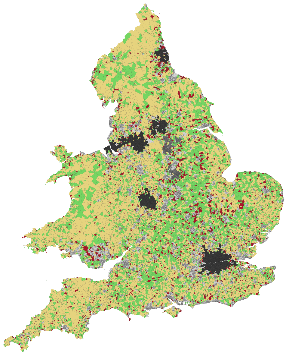
See Map 1 for a rural-urban classification breakdown of England and Wales.
Why can national comparisons be misleading?
A national comparison shows how a location compares with all Output Areas in England and Wales. This can be useful, but it does not always give the most relevant context.
This is because different types of places have different typical levels of connectivity. Dense urban areas usually score higher than rural areas because they tend to have more destinations and transport options nearby.
For example:
- a rural location may score below the national average, but still be highly connected for a rural area;
- an urban location may score above the national average, but still be poorly connected compared with similar urban areas.
For this reason, users should consider both the national comparison and the relevant rural-urban comparison.
What does each of the six rural-urban classifications mean?
The six classifications broadly describe different types of settlement, from the most dense urban places, to the least dense rural ones. See Table C below for individual descriptions.
| RUC 2011 | Classification Description | % of total Output Areas | Number of Output Areas |
|---|---|---|---|
| Urban Major Conurbation | There are six urban major conurbations. These are London, West Midlands, West Yorkshire, Tyneside, Merseyside and Greater Manchester. | 32.6% | 61,500 |
| Urban Minor Conurbation | There are two urban minor conurbations: Nottingham and South Yorkshire. | 3.4% | 6,418 |
| Urban City and Town | Built-up urban areas, with a minimum population of 10,000 inhabitants, which do not form part of major and minor conurbations. Commonly observed in areas such as Lincoln, Derby & York. | 45.0% | 84,958 |
| Rural Town and Fringe | Areas with fewer than 10,000 inhabitants, and associated with a larger neighbouring town. Commonly observed in areas of Northumberland, South Oxfordshire & Wiltshire. | 9.4% | 17,782 |
| Rural Village | Areas with fewer than 10,000 inhabitants, but with a denser physical form than in hamlets and isolated dwellings. Commonly observed in areas of Mid Suffolk & West Sussex. | 5.8% | 11,011 |
| Rural Hamlets and Isolated Dwellings | Areas with fewer than 10,000 inhabitants, dispersed housing, and no clear nucleated settlement. Commonly observed in areas of Cornwall & Carmarthenshire. | 3.8% | 7,211 |
Note: For more information about the methodology used for classifying Output Areas into the rural-urban classifications, see the Office for National Statistics guidance. See the What are Output Areas section for more detail on Output Areas.
How are the rural-urban classifications distributed across England and Wales?
Map 1 below shows a map of Output Areas in England and Wales, coloured by their rural-urban classification.
Map 1

How much do connectivity scores vary across rural-urban classifications?
Connectivity scores range from an average of 22.4 in “Rural hamlets and isolated dwellings”, to 77.1 in “Urban major conurbations”.
This shows how important it is to differentiate between different types of places.
Are there any limitations of the 2011 rural-urban classifications?
The 2011 classification is based on 2011 Census data, and therefore does not reflect recent development or changes in settlement patterns which could have changed an area’s rural-urban classification.
However, this is unlikely to materially affect the Connectivity Matrix. The urban major and minor conurbation classifications are largely fixed (relating to established conurbations like the West Midlands and London). The main possible change is in “Rural town and fringe” Output Areas becoming “Urban city and town” if they have grown above 10,000 people since 2011. As these areas make up a relatively small share of overall Output Areas, such changes are unlikely to alter the overall distribution significantly.
Users should therefore treat the classification as a useful guide, rather than a definitive judgement, and use it alongside local knowledge when interpreting connectivity scores.
There is a 2021 version of the rural-urban classifications, however, this was not chosen to be used to help interpret the connectivity scores as almost 75% of Output Areas fall into a single category, making it less useful for comparing connectivity across different types of places.
Can I see the rural-urban classification in the Connectivity Tool?
Rural-urban classifications are not currently displayed directly in the Connectivity Tool. This means that when a user selects a square, the tool does not currently show the rural-urban classification for that location.
This functionality may be added in a future update. Until then, users should use the supporting map and tables in this guidance, use the ONS links referenced in the How do I use the Connectivity Matrix section, and apply local knowledge as appropriate.
What are Output Areas?
Output Areas are small geographic areas used by the Office for National Statistics to publish census and related data.
Each Output Area typically contains between 40 and 250 households, with a resident population between 100 and 625 people.
The Connectivity Matrix uses Output Areas to calculate connectivity score thresholds as they are the smallest standard geography used for the rural-urban classifications, and provide a consistent geographic unit for comparing connectivity across England and Wales.
What is the local authority view within the Connectivity Tool?
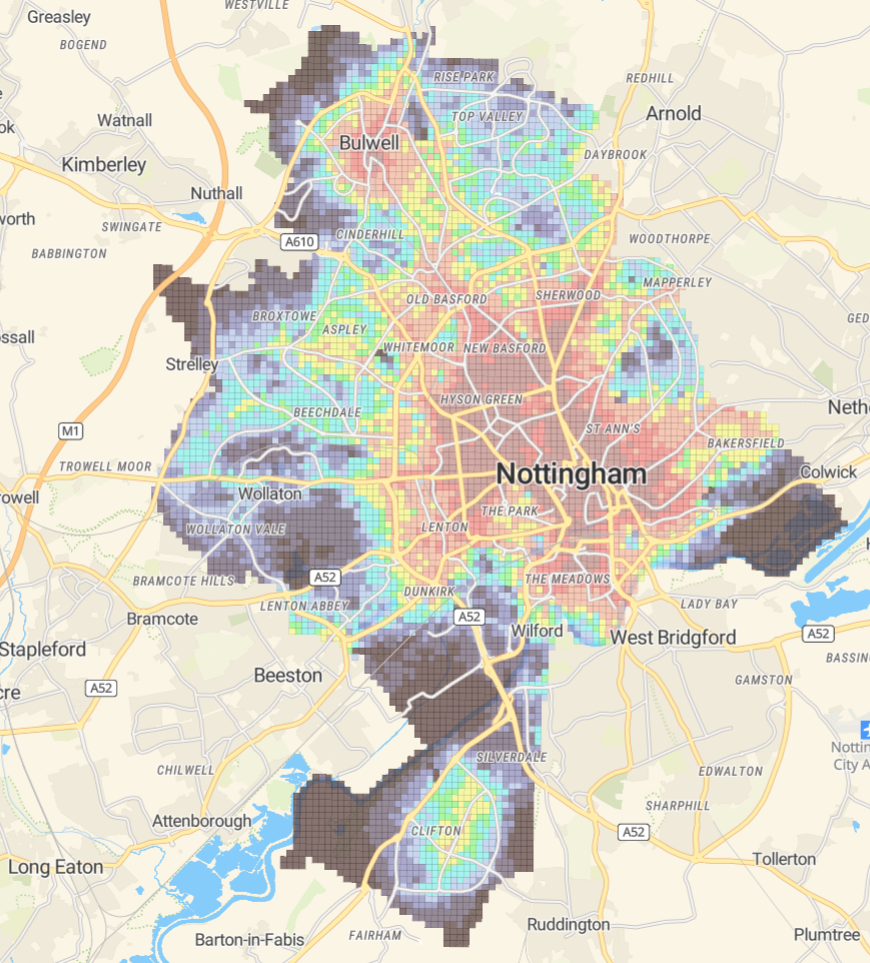
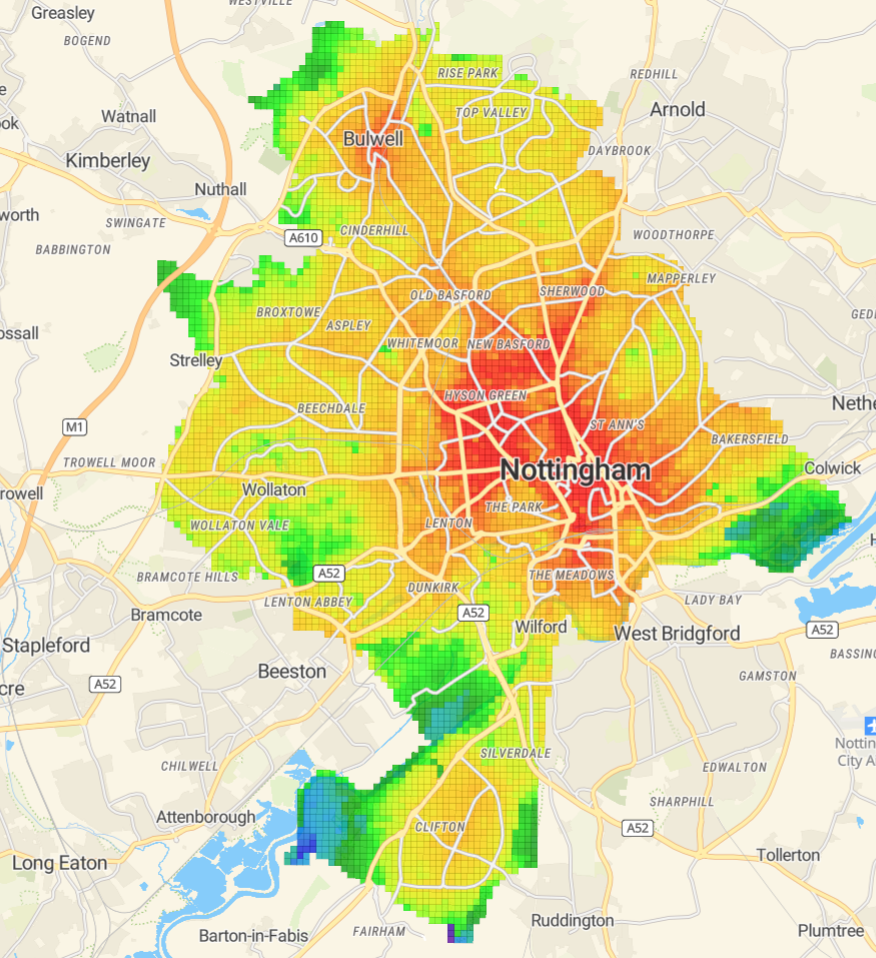
The local authority view groups connectivity scores within a selected local authority area and displays them in 10 colour bands. This can help users quickly see how connectivity varies across a specific area.
The colour bands are presented in Map 2. Map 3 has been added to demonstrate how local authority view differs from the default Connectivity Tool.
Map 2
Map 3
How should the local authority view be interpreted?
The local authority view only provides indicative connectivity differences. The bands are created by dividing all scores in the local authority into 10 equal groups, rather than reflecting meaningful thresholds of connectivity.
This means the local authority view should not be used on its own to inform decisions or draw firm conclusions. It is best used to get a quick, high-level sense of variation within an area, before using the connectivity scores and Connectivity Matrix for more robust interpretation.
Future updates to the tool may change how connectivity scores are presented.